Asymmetric measurements


< PREVIOUS: The metric system	_______________________________________________________> NEXT: The similarity score

Asymmetric similarity measurements are those where sound 1 is the model (or template) and sound 2 is the copy, and we want to judge how good the copy is in reference to the model. For example, if a bird has copied 4 out of 5 syllables in the song playbacks it has heard, we will say that 80% of the model was copied. However, what should we say had the bird produced a song of 10 syllables, including accurate copies of the 5 model syllables and 5 improvised syllables? It makes sense to state that all (100%) of the model song was copied, but the two songs are only 50% similar to each other. To capture both notions we will say that asymmetrically, the similarity to the model is 100%, and that symmetrically, the similarity between the two songs is 50%. We shall start with asymmetric comparisonsl

Start SAP2011, open 'Example 2' and outline the entire song. Click the 'Sound 2' tab, open 'Example 2' . For both sounds set amplitude threshold to 34dB to obtain a good segmentation to syllable units. Click the 'Similarity' tab and click 'Score'. The following image should appear within a few seconds (click the +/- zoom buttons to see the entire picture):

The gray level of the similarity matrix represents the Euclidean distances: the shorter the distance the brighter the color; intervals with feature distances that are higher than threshold are painted black. The numeric values of the similarity matrix are not useful to save in most cases, but those can be saved by checking the "Save similarity matrix" box. Then, after clicking score, a popup menu will prompt you to name the text file, where comma deliminated values of the matrix will be stored.

Similarity sections are neighborhoods of intervals that passed the threshold (e.g., when the corresponding p-value of Euclidean distance is less than 5% for all neighbors). Check 'Save detailed section matching' to have those sections automatically saved into the mySQL table 'similarity_sections'. As noted, the gray level represents the distance calculated for each pair of intervals. However the only role of the distance calculation across (70ms) intervals is to set a threshold based on 'viewing' features across a reasonably long interval. The actual similarity values are calculated frame-to-frame within the similarity section, where p-value estimates are based on the cumulative distribution of Euclidean distances across a large sample (250,000) of random pairs of frames obtained from comparisons across 25 random pairs of zebra finch songs. The gray level of the similarity matrix represents the Euclidean distances: the shorter the distance the brighter the color; intervals with feature distances that are higher than threshold are painted black.

Local (frame level) similarity scores: Based on this distribution, we can endow each pair of frames with a local similarity score, which is simply the complement of the Euclidean distance p-value. That is, if a single-frame p-value is 5% we say that the similarity between the two frames is 95%. Local similarity is encoded by colors in the similarity matrix as follows:

Score (1-p)%	Color
95-100	red
85-94	yellow
75-84	lime
65-74	green
50-64	olive
35-49	blue

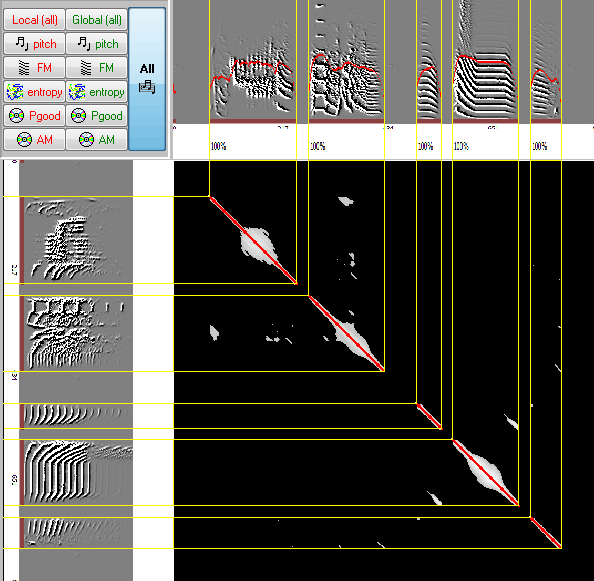
Section-level similarity Score: We now turn to the problem of estimating the overall similarity captured by each section. First, SAP2011 detects the boundaries of each section. Then, single frame scores are calculated for each pixel and finally, the algorithm searches for the best 'oblique cut' through the section, which maximizes the score. In the simplest case (e.g., of two identical sounds) similarity will maximize on a 45⁰ angle at the center of the section. In practice, it is not always the center of the section that gives the highest similarity, and the angle might deviate from 45⁰ if one of the sounds is time warped in reference to the other. We therefore need to expand in different displacement areas and at different angles. The default 'time warping tolerance' is set to 5% by default, allowing up to 5% angular deviation from the diagonal. Note that computation time increases exponentially with the tolerance. The search for best match is illustrated below:

We next consider only the frames that are on the best-matching diagonal, and calculate the average score of the section. This score is plotted above the section. Boundaries of similarity sections can be observed more clearly by clicking the 'Global' button. The light blue lines show the boundaries of each section and the rectangles enclose the best diagonal match of each section

Similarity across sections: Note that there are several sections with overlapping projections on both songs. To obtain a unique similarity estimate, we must eliminate redundancy by trimming (or omitting) sections that overlap with sections that explain more similarity. We call the former 'inferior sections' (blue rectangles) and the latter (red rectangle) 'superior sections'.

Final sections: once redundancy has been trimmed, it often makes sense to perform one final filtering, by omitting similarity sections that explain very little similarity (which are likely to be 'noise'). By default, SAP2011 omits sections that explain less than the equivalent of 10ms x 100% similarity. Superior similarity sections that passed this final stage are called final sections.