The SAP2011 data structure

How analysis results are stored in the database: SAP2011 automatically creates wave files and analyzes them. The results are saved in a database called SAP2011, where each table summarizes data of different types. Here is a brief description of the data tables according to their types:

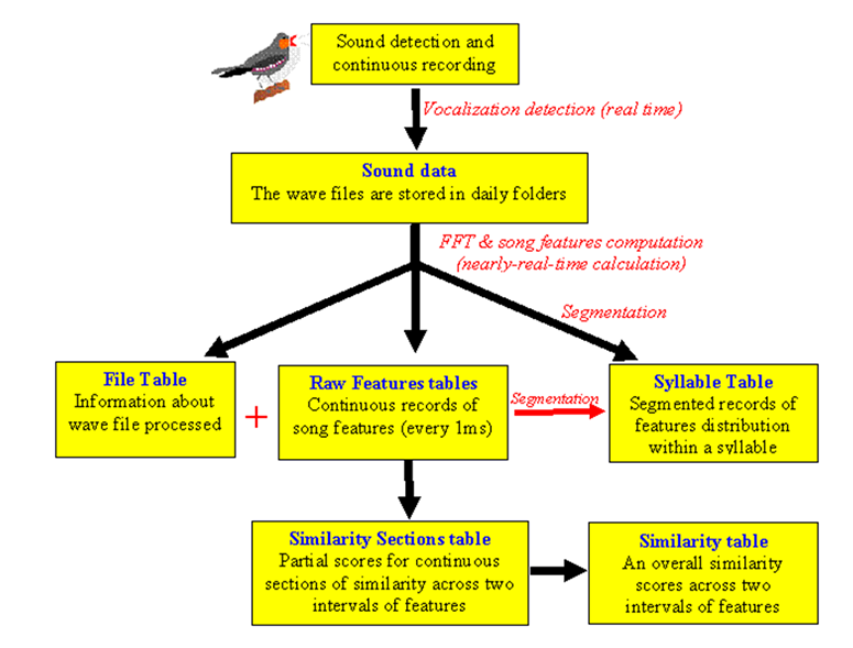The Sound Analysis Recorder detects vocalization and saves the sound data in wave files. Wave files are stored in daily folders. During recording, in nearly real time, the Sound Processing Live engine performs multi taper spectral analysis, and then computes the song feature. The features, usually computed in steps of 1ms, are stored in Raw Features tables. Note that these records are continuous, with no distinction between “silences” and “sounds”. By default, SAP2011 creates a single Raw Feature table per day, per bird. It is often a large table, including up to hundreds of millions of records. As the data from the (many) wave files flows into the Raw Features table, SAP2011 updates a small File Table, which contains indexes and file names of each processed wave file. Indexes for those wave files are saved in each of the Raw feature table records.The Raw Feature Table, together with the File Table, can be used to generate a Syllable Table. SAP2011 automatically create one Syllable Table that includes records of the entire song syllables the bird produced during an entire experiment.

The transition from Raw Feature Tables to the Syllable table is computationally cheap. However, segmentation of sound data is a difficult task, which you might want to revisit. This is one reason why it is useful to have the Raw Feature Tables - it is an analyzed version of your raw data that is still very raw. A second reason to have the Raw Feature Tables is that it is something meaningful to analyze sound data “as is” without any segmentation. Such analysis is particularly useful for so called “graded” signal, where segmentation is not necessarily meaningful and might induce artifacts. It is easy to compare raw features using the KS statistic.  The more complicated Similarity Measurements of SAP2011 are also based on raw features.

In the previous chapter we presented examples of how SAP2011 data can be exported easily to MS Excel. This method, however, is very  limited in its capacities and flexibilities. In order to take full advantage of SAP2011 you will need to understand some of its database structure and you will need to know how to access raw and processed data using using MySQL and Matlab. If you do not use Matlab it is recommended that you take a look at this chapter, and learn something about how to use MySQL to visualize and manipulate the data. If you do use Matlab, this chapter is very important, and also, we strongly recommend that you will learn just a little SQL (we will help you), which will help you to swiftly retrieve the appropriate data into matlab variables. In this chapter we present the database structure in a simplified manner. We then describe the structure of the feature tables, and show how those tables can be accessed in Matlab. SAP2011 raw data are saved as wave files, whereas all the derived data (features, similarity measures, clusters) are saved in a MySQL database tables.

SAP2 automatically generates tables of several different types, but you only need to know about some of them. Here is a simplified flowchart of what happens to sound data in SAP2011:

The SAP2011 recorder detects and save wave files into daily folders. Each daily folder might contain thousands of wave files. As wave files are recorded, “sound processing live” engine