Introduction to Spectral Analysis
| < PREVIOUS: Table of contents | > NEXT: Glossary of Terms |
|
|
|
|
This chapter presents some concepts of spectral analysis and acoustic features including some knowledge base that might help you get the most out of SAP2011. We will use the Explore & Score module to present those concepts. This module is similar to the previous versions of Sound Analysis with several new features. When listening to birdsong, it is immediately apparent that each song has a distinct rhythmic and sometimes even melodic structure. Songs of individual birds in a flock sound similar to each other and differ from those of other flocks. As early as the 18th century, Barrington noted that the songs of cross-fostered birds differed from the species-typical song, suggesting a role for vocal learning. However, until the late 1950s, there had been no objective way of confirming these observations by physical measurements of the songs themselves. The invention of the sound spectrograph (sonogram) at Bell Laboratories was a significant breakthrough for quantitative investigation of animal vocal behavior. The sonogram transforms a transient
stream of sound into a simple static visual image revealing the time-frequency structure of each song syllable. Sonogram images can be measured, analyzed, and compared with one another. This allows the researcher to quantify the degree of similarity between different songs by inspecting (or cross-correlating) sonograms and categorizing song syllables into distinct types. Each song is then treated as a string of symbols, corresponding to syllable types, e.g., a, b, c, d..., and song similarity is estimated by the proportion of shared syllable types across the sonograms of the two songs. The procedure is equally useful in comparing the songs of different birds and that of the same bird at different ages or after control and experimental treatments.
Spectral analysis is less than intuitive, and here is a little technical tutorial about how sonograms are computed:
When recording a singing bird, the microphone capture tiny fluctuations in air pressure we call sound waves and turn those into an electrical current, which might look like this over 20 milliseconds: 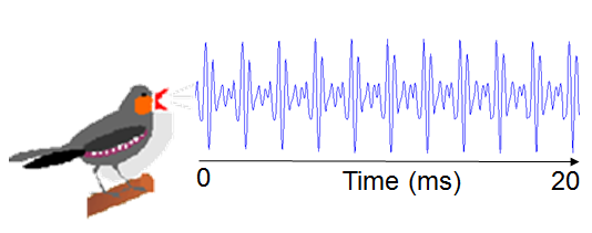 The fast Fourier transform (FFT) is an algorithm to compute the periodic structure in the signal, but representing it by a set of sine waves, called frequencies. Plotting the power of each one of those frequencies gives the Power Spectrum:

Each of of the peaks in the Power Spectrum above, corresponds to a sine wave, e.g.,:
 Now comes the interesting part: if we take those waves and add them, we will get a combo wave that looks like this:
 Exactly like the original wave, that is, the Power Spectrum (including phase, that is usually not shown) is a complete representation of the sound. We can look at the time domain (wave form) or frequency domain (the Power spectrum), and it summarizes its periodic structure.
Computing power spectrum works best when the signal is periodic and stationary, which is why in sound it usually makes sense to use short time windows, e.g., 5-20ms. To look at an entire song we have to summarize power spectra of many small time windows. This is how it is done: Take the power spectrum of one window, say from the first 20ms of the song, flip it and replace the graph with a color bar:
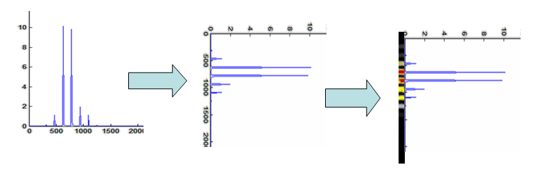 and now repeat this procedure for overlapping time windows, i.e., 1-20ms, 2-21ms, 3-22, etc, and stack the color bars next to each other. The outcome might look like this:
 This is the famous sonogram! It is a set of vertical strips, each one represent the power spectrum of one time window of sound.
|
|